
Last week, I needed to mail some stuff to one of my friends who recently moved to a new city. So, I called him to inquire about his new address. During the phone call, I quick jotted down the address on a piece of paper and then we took an expected discourse on topics running the entire gamut from movies to politics. After finishing the telephonic conversation, when I gazed at the address that I wrote, it took me a while to understand my own handwriting. I still vividly remember when I was in high school, my mathematics teacher gave me a zero in one of the problems in the test, simply because she was unable to decipher my oracular calligraphy 🙂 , quite an oxymoron . Those were really tough times! Subsequently, I thought about training a classifier to recognize my handwriting. After a couple of days piecemeal work, I was able to recognize my handwriting. Although, I did not do a quantitative analysis of the results, they were all but satisfactory. This motivated me to write a blog post on detecting handwritten digits using HOG features and a multiclass Linear SVM.
Before we begin, I will succinctly enumerate the steps that are needed to detect handwritten digits –
- Create a database of handwritten digits.
- For each handwritten digit in the database, extract HOG features and train a Linear SVM.
- Use the classifier trained in step 2 to predict digits.
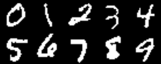
MNIST database of handwritten digits
The first step is to create a database of handwritten digits. We are not going to create a new database but we will use the popular MNIST database of handwritten digits. The MNIST database is a set of 70000 samples of handwritten digits where each sample consists of a grayscale image of size 28×28. There are a total of 70,000 samples. We will use sklearn.datasets package to download the MNIST database from mldata.org. This package makes it convenient to work with toy datasbases, you can check out the documentation of sklearn.datasets here.
The size of of MNIST database is about 55.4 MB. Once the database is downloaded, it will be cached locally in your hard drive. On my Linux system, by default it is cached in ~/scikit_learn_data/mldata/mnist-original.mat . Alternatively, you can also set the directory where the database will be downloaded.
There are approximate 7000 samples for each digit. I actually calculated the number of samples for each digit using collections.Counter class. The actual samples for each digit was –
| Digits | Number of samples |
|---|---|
| 0 | 6903 |
| 1 | 7877 |
| 2 | 6990 |
| 3 | 7141 |
| 4 | 6824 |
| 5 | 6313 |
| 6 | 6876 |
| 7 | 7293 |
| 8 | 6825 |
| 9 | 6958 |
We will write 2 python scripts – one for training the classifier and the second for test the classifier.
Also Read: Best Processor Under 10000
Training a Classifier
Here, we will implement the following steps –
- Calculate the HOG features for each sample in the database.
- Train a multi-class linear SVM with the HOG features of each sample along with the corresponding label.
- Save the classifier in a file
The first step is to import the required modules –
1
2
3
4
5
6# Import the modules
from sklearn.externals import joblib
from sklearn import datasets
from skimage.feature import hog
from sklearn.svm import LinearSVC
import numpy as np
We will use the sklearn.externals.joblib package to save the classifier in a file so that we can use the classifier again without performing training each time. Calculating HOG features for 70000 images is a costly operation, so we will save the classifier in a file and load it whenever we want to use it. As discussed above sklearn.datasets package will be used to download the MNIST database for handwritten digits. We will use skimage.feature.hog class to calculate the HOG features and sklearn.svm.LinearSVC class to perform prediction after training the classifier. We will store our HOG features and labels in numpy arrays. The next step is to download the dataset using the sklearn.datasets.fetch_mldata function. For the first time, it will take some time as 55.4 MB will be downloaded.
1dataset = datasets.fetch_mldata("MNIST Original")
Once, the dataset is downloaded we will save the images of the digits in a numpy array features and the corresponding labels i.e. the digit in another numpy array labels as shown below –
1
2features = np.array(dataset.data, 'int16')
labels = np.array(dataset.target, 'int')
Next, we calculate the HOG features for each image in the database and save them in another numpy array named hog_feature.
1
2
3
4
5list_hog_fd = []
for feature in features:
    fd = hog(feature.reshape((28, 28)), orientations=9, pixels_per_cell=(14, 14), cells_per_block=(1, 1), visualise=False)
    list_hog_fd.append(fd)
hog_features = np.array(list_hog_fd, 'float64')
In line 17 we initialize an empty list list_hog_fd, where we append the HOG features for each sample in the database. So, in the for loop in line 18, we calculate the HOG features and append them to the list list_hog_fd. Finally, we create an numpy array hog_features containing the HOG features which will be used to train the classifier. This step will take some time, so be patient while this piece of code finishes.
Also Read: Best Gaming Laptops Under 35000 In India
To calculate the HOG features, we set the number of cells in each block equal to one and each individual cell is of size 14×14. Since our image is of size 28×28, we will have four blocks/cells of size 14×14 each. Also, we set the size of orientation vector equal to 9. So our HOG feature vector for each sample will be of size 4×9 = 36. We are not interesting in visualizing the HOG feature image, so we will set the visualise parameter to false.
If you don’t know about Histogram of Oriented Gaussians (HOG), don’t be disappointed because it is pretty easy to understand. You can check out the below 16 minute YouTube video by Dr. Mubarak Shah from UCF CRCV. Alternatively, you can check out the documentation of the skimage’s hog function from the official page. They do discuss tersely about how HOG works.
The next step is to create a Linear SVM object. Since there are 10 digits, we need a multi-class classifier. The Linear SVM that comes with sklearn can perform multi-class classification.
1clf = LinearSVC()
We preform the training using the fit member function of the clf object.
1clf.fit(hog_features, labels)
The fit function required 2 arguments –one an array of the HOG features of the handwritten digit that we calculated earlier and a corresponding array of labels. Each label value is from the set — [0, 1, 2, 3,…, 8, 9]. When the training finishes, we will save the classifier in a file named digits_cls.pkl as shown in the code below –
1joblib.dump(clf, "digits_cls.pkl", compress=3)
The compress parameter in the joblib.dump function is used to set how much compression is done and I am quoting this from the documentation –
compress: integer for 0 to 9, optional
Optional compression level for the data. 0 is no compression. Higher means more compression, but also slower read and write times. Using a value of 3 is often a good compromise.
Up till this point, we have successfully completed the first task of preparing our classifier.
Testing the Classifier
Now, we will write another python script to test the classifier. The code for the second script is pretty easy and here is the code for the same –
1
2
3
4
5
6
7
8
9
10
11
12
13
14
15
16
17
18
19
20
21
22
23
24
25
26
27
28
29
30
31
32
33
34
35
36
37
38
39
40
41
42
43
44
45# Import the modules
import cv2
from sklearn.externals import joblib
from skimage.feature import hog
import numpy as np

# Load the classifier
clf = joblib.load("digits_cls.pkl")

# Read the input image
im = cv2.imread("/home/bikz05/Desktop/photo8.jpg")

# Convert to grayscale and apply Gaussian filtering
im_gray = cv2.cvtColor(im, cv2.COLOR_BGR2GRAY)
im_gray = cv2.GaussianBlur(im_gray, (5, 5), 0)

# Threshold the image
ret, im_th = cv2.threshold(im_gray, 90, 255, cv2.THRESH_BINARY_INV)

# Find contours in the image
ctrs, hier = cv2.findContours(im_th.copy(), cv2.RETR_EXTERNAL, cv2.CHAIN_APPROX_SIMPLE)

# Get rectangles contains each contour
rects = [cv2.boundingRect(ctr) for ctr in ctrs]

# For each rectangular region, calculate HOG features and predict
# the digit using Linear SVM.
for rect in rects:
    # Draw the rectangles
    cv2.rectangle(im, (rect[0], rect[1]), (rect[0] + rect[2], rect[1] + rect[3]), (0, 255, 0), 3)
    # Make the rectangular region around the digit
    leng = int(rect[3] * 1.6)
    pt1 = int(rect[1] + rect[3] // 2 - leng // 2)
    pt2 = int(rect[0] + rect[2] // 2 - leng // 2)
    roi = im_th[pt1:pt1+leng, pt2:pt2+leng]
    # Resize the image
    roi = cv2.resize(roi, (28, 28), interpolation=cv2.INTER_AREA)
    roi = cv2.dilate(roi, (3, 3))
    # Calculate the HOG features
    roi_hog_fd = hog(roi, orientations=9, pixels_per_cell=(14, 14), cells_per_block=(1, 1), visualise=False)
    nbr = clf.predict(np.array([roi_hog_fd], 'float64'))
    cv2.putText(im, str(int(nbr[0])), (rect[0], rect[1]),cv2.FONT_HERSHEY_DUPLEX, 2, (0, 255, 255), 3)

cv2.imshow("Resulting Image with Rectangular ROIs", im)
cv2.waitKey()
From line 2-5 we load the required modules. In line 8, we load the classifier from the file digits_cls.pkl __which we had saved in the previous script. In __line 11, we load the test image and in line 14 we convert it to a grayscale image using cv2.cvtColor function. We then apply a Gaussian filter in line 15 to the grayscale image to remove noisy pixels. In line 18, we convert the grayscale image into a binary image using a threshold value of 90. All the pixel locations with grayscale values greater than 90 are set to 0 in the binary image and all the pixel locations with grayscale values less than 90 are set to 255 in the binary image. In line 21, we calculate the contours in the image and then in line 24 we calculate the bounding box for each contour. From line 28-35 for each bounding box, we generate a bounding square around each contour. Then in line 37, we then resize each bounding square to a size of 28×28 and dilate it in line 38. In line 40, we calculate the HOG features for each bounding square. Remember here that the HOG feature vector for each bounding square should be of the same size for which the classifier was trained, else you will get an error. In line 41, we predict the digit using our classifier. We also draw the bounding box and the predicted digit on the input image. Finally, in line 44 we display the image.
Also Read: Best Laptops Under 1 Lakh In India
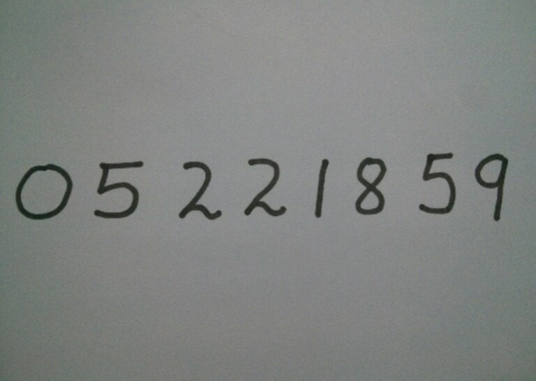
I tested the classifier on this image –
The resulting image, after running the second script was –
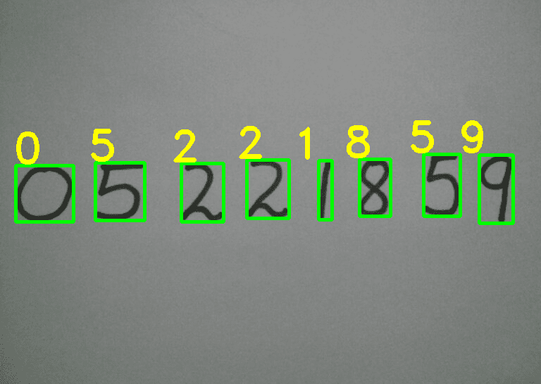
So, the results are pretty good.
Here is another result –
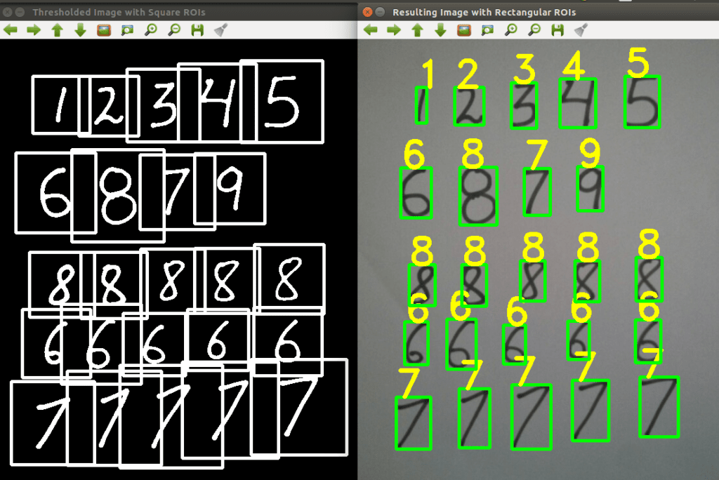
(Above) In the image on the left hand side, we display the thresholded image with a square around each digit. Each of this square region is then resized to a 28×28 image. After resizing, we calculate the HOG features of this square region and then using these HOG features we predict the digit. In the image on the right hand side, we display the predicted digit for each handwritten sample bounded in the rectangular box.
Assumption during testing
There are a few assumptions, we have assumed in the testing images –
- The digits should be sufficiently apart from each other. Otherwise if the digits are too close, they will interfere in the square region around each digit. In this case, we will need to create a new square image and then we need to copy the contour in that square image.
- For the images which we used in testing, fixed thresholding worked pretty well. In most real world images, fixed thresholding does not produce good results. In this case, we need to use adaptive thresholding. You can check out this blog post on adaptive thresholding that I wrote some weeks back.
- In the pre-processing step, we only did Gaussian blurring. In most situations, on the binary image we will need to open and close the image to remove small noise pixels and fill small holes.
Recap
In this tutorial, we discussed how we can recognize handwritten digits using OpenCV, sklearn and Python. We trained a Linear SVM with the HOG features of each sample and tested our code on 2 images. So, That’s it for now!! I hope you liked this blog post.